Alasdair’s Engineering Pages © A. N. Beal 2025             www.anbeal.co.uk

www.anbeal.co.uk

Proc. Instn. Civ. Engrs Structs & Bldgs, 1999, 134, Nov., 345-357

Paper 11847

Design of normal- and high-strength concrete columns

A. N. Beal, BSc, CEng, MICE, MIStructE

(Associate, Thomason Partnership, Leeds) and

N. Khalil, BSc, PhD, MACI, MASCE

Assistant Professor, Department of Civil Engineering, University of Balamand, Tripoli, Lebanon)

Research by Khalil to verify and develop Beal’s graphical method of buckling analysis confirms that Beal's method is accurate and effective, giving results which agree well with experimental data. The method provides a powerful analytical tool, allowing fast determination of the column capacity for a wide range of slenderness and loading conditions. It is used here to investigate the behaviour of normal- and high-strength concrete columns under both axial and eccentric loads and with a variety of slenderness ratios and reinforcement proportions. The results of this accurate analysis are used as a benchmark for the assessment of code of practice design rules. Existing BS 8110 design rules are found to give poor agreement with both the theoretical analysis and experimental results. New design rules which give more consistent and accurate results are proposed.

Keywords: buildings, structure & design; columns; concrete structures

Introduction

The analysis of slender reinforced concrete columns is complicated because the buckling analysis must take account of the non-linear properties of the materials and also construction imperfections. Exact analysis methods are generally complicated and unsuitable for everyday design. Codes of practice recommend various design methods for slender columns based on capacity reduction factors, additional design moments, or moment magnification, to account for the effects of buckling. These methods are approximate and largely empirical in nature. There is now considerable interest in the use of high-strength concrete in columns, which can allow columns that are more slender to be used to sustain high loads. Therefore one of the objectives of the present study is to investigate the theoretical behaviour of such columns, in order to establish suitable rules for their design.

2. A simple graphical technique has been proposed by Beal for rigorous analysis of pin-ended slender reinforced concrete columns [1]. Firstly, graphs of load eccentricity against section curvature are prepared for various values of applied axial load. Then a second set of graphs is prepared which plot the deflected shape of the column as it buckles, relating its mid-height deflection to the maximum section curvature. The deflection is calculated assuming a sine curve for the deflected shape of the column

Δ/h = (1/π²)(L/h)²(h/R)                                    (1)

where Δ is the deflection, L is the column effective length, h is the column width in the direction of buckling and R is the radius of curvature. By overlaying the two graphs, the section capacity can be established (see Fig. 1). Once section moment-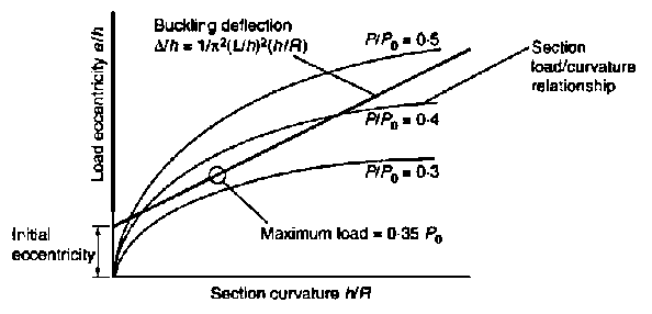curvature relationships are established, this technique allows rapid determination of column capacity under any combination of slenderness ratio and initial eccentricity.

Fig. 1. Overlay of graphs to establish slender column and capacity

3. Beal’s original paper set out the theoretical basis of the graphical analysis method. Design recommendations were presented for columns made from normal-strength concrete (up to 50 N/mm² cube strength) and it was shown that these gave better agreement with test results than existing UK codes of practice. Compared with Cranston’s long-term test results [2] Beal’s analysis gave ratios (Ptest/Ptheory) of 0.97-1.97, with a mean of 1.28 and a coefficient of variation of 0.16, a considerable improvement over existing design methods (see later). In the discussion of Beal’s paper [3], Drs Maisel and Beeby showed that a computer program devised by Cranston for nonlinear buckling analysis gave very similar results to the graphical analysis, for both peak load and column deflection (see Figs 12 and 13 in Reference 3). In the same discussion, Dr Wong described an alternative graphical analysis method which he and Professor Kong have developed; he confirmed that in his opinion this should also give similar results.

4. At Leeds University, Dinku [4] investigated the proposed analytical method in the light of existing experimental data reviewed by Cranston. Dinku developed computer programs to generate load eccentricity-curvature graphs in terms of capacity ratio (P/P0), based on stress-strain relationships for concrete and steel. His research verified that the graphical analysis method predicts the capacity of concentrically or eccentrically loaded pin-ended slender columns quickly and accurately.

5. The work of Beal and Dinku encouraged further research by Khalil, which is summarized here. Following her verification of the accuracy of the graphical analysis method, it was used to carry out a comprehensive theoretical investigation of the behaviour of reinforced concrete columns made from both normal- and high-strength concrete. The effects of creep, cracking, initial imperfections and non-linear stress-strain curves were all taken into account in the analysis, which covered a wide range of load eccentricities and also the full practical range of column slenderness. The results from existing (BS 8110) design rules were compared with the answers from the accurate analysis. The results from the accurate analysis were then used as a benchmark for developing new design recommendations for both normal- and high-strength concrete columns. These new design recommendations give more consistent and reliable results.

Research by Khalil

6. The computer programs developed by Dinku to generate graphs for eccentricity against curvature for different capacity ratios (P/P0) were limited in their application and were based on CP 110 stress-strain relationships for concrete and steel. Therefore it was necessary to generalize these programs to deal with different locations of reinforcement and to take account of long-term effects and also to update them using the BS 8110 stress-strain diagrams for concrete and steel.

7. In the test programme, eleven reinforced concrete columns with slenderness ratios between 18 and 63 were tested under short-term load and eight similar columns tested under sustained load. Details of the experimental investigation including descriptions of test columns, concrete properties, test procedures and discussion of the observations made are fully covered elsewhere [6, 7]. In these tests, the experimental buckling load and mid-height eccentricity at the point of instability were measured and compared with theoretical predictions (Table 1).

8. In the long-term tests, a load of 60% of short-term failure load was applied to 28-day old columns and maintained for a period of 90 days. If at the end of this period the column had not failed, it was then subjected to an increasing short-term load until failure. Applying this short-term load at the end of the loading period will tend to produce a rather higher apparent strength than if the entire load were long term, so the tests indicate a good agreement between the theoretical predictions and experimental results. Close agreement was also obtained between theoretical and actual column deflections at failure.

9. To provide a general indication of the validity and accuracy of the proposed theory, comparisons with other published tests were carried out. These are shown in Table 2.

The BS 8110 method

10. It should be noted that the ‘additional moment’ theory used for slender column design in BS 8110 [12] is open to serious theoretical objections (see paras. 79-82 of Reference 3).

11. BS 8110 estimates the buckling deflection of a column at failure on the basis that

(a) the maximum concrete compressive strain is 0.0035;

(b) the maximum steel tensile strain is 0.002;

(c) initial imperfections are allowed for by an initial eccentricity of 0.05h unless the applied moment exceeds this, in which case the allowance for imperfections is zero at higher compressive stresses;

(d) the assumed buckling deflection is reduced using an interaction formula by a factor K, on the assumption that the steel tensile strain at failure will not exceed 0.002.

12. Based on this estimate of column buckling deflection, an additional moment is calculated which is added to the applied design moment and the column section is then designed to resist the total combined moment. The section strength is calculated on the basis of full plasticity, with a maximum concrete strain of 0.0035 and allowable steel strains in excess of yield.

13. However, the following points should be noted.

(a) Buckling failure in a slender column typically occurs at stresses and strains well below the values associated with fully plastic material failure.

(b)  As noted earlier, the assumed concrete strain limit of 0.0035 is for short-term loads; under long-term loading (which is more relevant to real structures), creep increases the maximum strain to two to three times this value.

(c) For 460N/mm² steel reinforcement, the tensile strain at yield is 0.0023 - not 0.002 as assumed - and in any case the reinforcement can be stressed past its yield point, developing strains far in excess of 0.002.

(d) The ‘flat rate’ allowance of 0.05h to cover initial imperfections in an axially loaded column is too crude and it is a mistake to ignore the effects of initial imperfections on the strength of an eccentrically-loaded column.

14. It is strange that the BS 8110 additional moments are calculated on the assumption that the steel tensile strain is always less than its elastic limit (0.002) whereas the concrete compressive strain is taken up to its plastic limit (0.0035). To compound the problem, these moments are then applied to a section whose strength is calculated on the assumption that both the steel and the concrete can be stressed right up to their plastic limits. Then the calculation is done on the basis of short-term material properties, despite the fact that real columns carry long-term loads. Thus the BS 8110 analysis is not based on a consistent, logical assessment of column behaviour in either elastic or plastic conditions. The failure to allow properly for the effects of creep is a serious omission.

15. Some of the assumptions underlying the BS 8110 method are very conservative but others are over optimistic. Therefore when compared with an accurate rigorous analysis, the results are likely to vary unpredictably, being over-conservative in some cases and possibly unsafe in others. Most published comparisons between the BS 8110 method and test results consider only short-term tests and these often show reasonable correlations, albeit with high coefficients of variation. However, comparisons with long-term test results (which are more relevant to real design) show that, in tests, a disturbing number of failures have occurred at loads well below those predicted by the code. Cranston’s original report on the development of the code design method included a table of experimental results from long-term load tests and in Reference 1 these were compared with the results from CP 110 (which is very similar to BS 8110) and Beal’s analysis. The results are summarized in Table 3. As can be seen, the CP 110 method gave poor prediction of experimental results, with a high coefficient of variation and test columns failing at as little as 56% of the predicted load. Beal’s analysis gave much better results, with a reduced coefficient of variation and test ‘failures’ almost eliminated.

16. It should be noted that the draft Eurocode EC2 for concrete design adopts a different formulation of the ‘additional moment’ method from BS 8110. The EC2 treatment is more logical in some respects, particularly its treatment of initial imperfections (where the initial imperfection is taken as L/400) and when compared with an accurate theoretical analysis it gives more consistent and reasonable results than BS 8110 [13]. However, it still lacks the firm logical basis that is an essential requirement for any important structural calculation.

17. In principle, the problems identified in the BS 8110 method could be dealt with by recalculating the additional moments to take proper account of steel post-yield behaviour and concrete creep to give appropriate values for use with plastic ultimate section strength but the results would be extremely conservative and unlikely to be acceptable. The problem is that by the time that a column develops its full plastic moment resistance at mid-height, it has usually buckled so badly that it can carry very little load.

18. As an alternative, both the buckling deflection and the section strength could be calculated on the basis of elastic theory. This would be more logical and appropriate, as buckling usually occurs at stresses which are in the elastic range, so an elastic analysis would probably give better results than plastic theory. However, the results would still be conservative and concrete designers would need to relearn elastic theory, which is distinctly unfashionable among present-day engineers.

19. The problem is that the buckling behaviour of a reinforced concrete column is too complex to be accurately modelled by a simple theoretical analysis. To achieve better results than present-day codes, a semi-empirical approach is the most realistic way forward. It would be difficult and costly to test all possible types of column and loading in the laboratory. However, if a practical, accurate method of theoretical analysis is established and proved to give satisfactory results, it is then possible to carry out a comprehensive investigation of column behaviour and the effects all the various factors can have on column strength can be analysed and quantified. The results of the accurate theoretical analysis will then provide a benchmark against which the results from various design rules can be assessed and the design methods can be optimised by adjusting the values of key parameters in order to give the best results.

Safety factors

20. Before proceeding further, it should also be noted that there are problems in applying the partial factor system favoured by current limit state codes to the analysis and design of slender concrete columns. Codes such as BS 8110 and EC2 divide the structure's safety factor into two parts: a load factor γL applied to loads; and a materials factor γm applied to the material strength (e.g. concrete cube strength or steel yield stress). However, Young’s modulus for concrete is proportional only to the square root of the cube strength and for steel it does not vary with yield stress at all. Thus in these codes there is effectively only a reduced partial safety factor applied to concrete stiffness and no factor at all on the stiffness of reinforcing steel. As the strength of a slender column depends primarily on its stiffness, BS 8110’s partial factor theory would lead to the conclusion that a slender column should have a lower safety factor than a stocky column, which is surely wrong.

21. Buckling failure can occur suddenly, with little warning and minimal scope for beneficial redistribution of load and there is a strong case for saying that the safety factor against this type of failure should be at least as high as that for other more ductile failure modes such as flexural bending. To achieve a consistent safety factor, it is necessary to adopt either a global overall safety factor on the column strength (as used in permissible stress codes), or, if partial factors are to be used, the ‘materials’ factor should be applied to the member strength (as in the American ‘resistance factor’) rather than to the material strength (as in the BS 8110 and EC2 ‘materials factors’).

22. (It should be noted that only part of BS 8110’s ‘material factor’ for 1.5 on concrete should be considered as a safety factor. Because of inferior placing and curing conditions, concrete in real structures has typically only about 75% of the strength of laboratory test cubes [14]. The effective safety factor on concrete in a real BS 8110 design is thus about 1.5 x 0.75 = 1.12,which compares with the steel partial factor of 1.15 (reduced to 1.05 in the most recent revision of BS 8110).)

Analysis of normal- and high-strength concrete columns

23. Following the research work by Khalil outlined earlier, the graphical analysis method was used to investigate slender column behaviour over the full realistic range of concrete strengths, including high-strength concrete. The theoretical column load capacity was calculated for a wide range of slenderness ratios and load eccentricities, taking into account the effects of initial imperfections and concrete creep.

24. The analysis covered concrete cube strengths from 20 N/mm² to 100 N/mm². The BS 8110 [12] stress-strain curve (Fig. 2) was used to define concrete short-term behaviour, but for concrete with cube strengths over 60 N/mm² the peak compressive strain was limited to ξ = 0.0035 - ((fcu - 60)/50,000). As columns in real structures generally support predominantly long-term loads, this was the condition considered in the analysis. The concrete short-term stress-strain curve was modified for long-term loading by the creep factor φ, with a value of 2.0 for cube strengths up to 30 N/mm². For higher concrete strengths this was reduced to φhsc = φ√(40/(fcu + 10)), giving creep factors ranging from 2.00 for 20 N/mm² concrete to 1.21 for 100 N/mm² concrete. Combining the various factors, the concrete ultimate long-term compressive failure strain ranged from 0.0105 for 20 N/mm² concrete to 0.00595 for 100 N/mm² concrete.

Fig. 2. Short-term design stress-strain curve for normal-  weight concrete according to BS 8110: Part 1 (fcu is in N/mm²)

25. Steel behaviour was assumed to follow the BS 8110 stress-strain curve (see Fig. 3) and allowance was made in the analysis for displacement of concrete by the steel. The section calculations were based on a 4 bar reinforcement arrangement with d = 0.8h, which should reasonably cover most real columns without being unduly conservative.

Fig. 3. Short-term design stress-strain curve for reinforcement according to BS 8110: Part 1 (fy is in N/mm²)

26. Calculations were run using a spreadsheet which was developed to run on Lotus 123 or Microsoft Works to calculate the moment-curvature relationship for each section at various values of axial load. This spreadsheet is designed to allow any value of concrete strength, creep factor or concrete peak strain to be inserted, reinforcement effective depth to be varied and either 4 bar or 6 bar reinforcement arrangements considered. To use the spreadsheet, material properties and a value of peak concrete strain are first selected and then the neutral axis position is varied (by trial and error) until the load eccentricity and curvature are shown which correspond to the required value of axial load (P = 0.1P0, 0.2P0, etc., where P0 is the section ultimate compressive strength). By repeating the calculations for a range of neutral axis positions and peak strain values, families of curves can be generated which define the section flexural behaviour under different axial loads.

27. The allowance for column initial imperfections was taken as an initial bow of 0.002L, which in the absence of better information was felt to be a reasonable value for use in practical design. This is equivalent to an initial bow of 6 mm on a braced 3m column, or 12 mm out of plumb on a 3m unbraced column.

28. As previously described, graphs were prepared, plotting the results of the section behaviour calculations as load eccentricity (e/h) against section curvature (h/R) for various values of axial load P (expressed as a proportion of the section strength in pure compression, P0). Another graph was then prepared (on tracing paper) showing the relationship between buckling deflection and section curvature for various slenderness ratios, assuming that the buckled shape of the column follows a sine curve: Δ/h = (L/h)²(h/R)/π² (see equation (1)). By overlaying this buckling deflection graph on the section behaviour graphs, the column capacities for various slenderness ratios could be read off directly.

29. As noted earlier, where applied moments are significant, for an exact solution an iterative approach is required which takes into account the difference between the circular curvature induced by the applied end moments and the sinusoidal curvature induced by buckling. The deflection induced by circular curvature is

Δ/h = (L/h)²(h/R)/8                      (2)

The results presented in this paper have all been calculated by the exact iterative method.

30. The results of the theoretical analysis are summarized in Tables 4-8 (Figs 4-8 refer). These are expressed as the ratio of slender column capacity to short column ‘squash’ capacity (P/P0). These results show the effect that buckling and initial imperfections have on the load capacity (with no safety factors applied) for each column analysed. They give a precise analytical benchmark against which proposed design methods for slender columns can be assessed.

31. In carrying out the analysis, one interesting point was apparent at the outset: when high strength concrete is used, an eccentrically loaded section may be able to carry a greater long-term load than its short-term capacity, because the concrete’s limited short-term strain capacity restricts the steel stress which can be developed. As it is usual to calculate the strength of a reinforced concrete section on the basis of short-term loading, short-term section strengths have been used for the comparisons in Tables 4-8.

Fig. 4. Relationship between slender column capacity L/h and short column ‘squash’ capacity PIP,, for: (a) 20 N/mm², r = 0.8%; and (b) 20 N/mm² and r = 4%

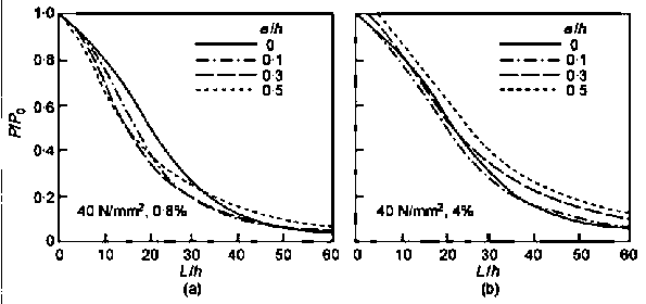
Fig. 5. Relationship between slender column capacity, Llh and and short column ‘squash’ capacity P/P0 for: (a) 40N/mm², r = 0.8%; and (b) 40 N/mm², r = 4%

Fig. 6. Relationship between slender column capacity L/h and short column ‘squash’ capacity P/P0 for: (a) 60 N/mm², r = 0.8%; and (b) 60 N/mm², r = 4%

Fig. 7. Relationship between slender column capacity L/h and short e column ‘squash’ capacity P/P0 for: (a) 80 N/mm², r = 0.8%; and (b) 80 N/mm², r = 4%

Fig. 8. Relationship between slender column capacity L/h and short column ‘squash’ capacity P/P0 for: (a) 100 N/mm², r = 0.8%; and 100 N/mm², r = 4%

Revising BS 8110

32. A comparison between the results of the accurate analysis and designs in accordance with the BS 8110 rules is presented in Table 9(a) and Fig. 9(a) and Table 9(b) and Fig. 9(b). (The ratios give the strength of the slender column relative to that of a column with L/h = 0.) This is done for an axially loaded column made from 80 N/mm² concrete, with r = 0.8% and 4%, taking into account the additional moment for buckling in the BS 8110 calculation, and also the factor K which reduces this at high axial loads. The optimum value of K has been calculated iteratively in accordance with BS 8110. A K = 1 line is also shown added in Tables 9(a) and (b) to show the effect of setting the factor K as a constant 1.0, instead of being reduced by iteration.

33. As can be seen, the BS 8110 ‘exact’ analysis overestimates the strength of a column with 0.8% steel by up to 95% and for 4% steel it overestimates the strength by up to 80%. The worst problems are with slenderness ratios around L/h = 20, where the BS 8110 factor K acts to eliminate buckling effects from the calculation, leading to a calculated column strength which is far in excess of the true value. If setting  K = 1 in all cases, the results from the BS 8110 become more realistic but still  the column strength is overestimated by 30% for slenderness ratios of 10 and above.

Fig. 9. BS 8110 comparison for: (a) 80 N/mm², r = 0.8%; and
(b) 80 N/mm², r = 4%

34. Table 10 shows the adjusted values of additional load eccentricity (including allowance for initial imperfections) which would be required to give results which agree with the rigorous theoretical analysis. As can be seen, the additional eccentricities which are required to match the results of the accurate  analysis are generally higher than the present values recommended in BS 8110. However, it is interesting that for axially loaded columns with slenderness up to L/h = 25, the required value of additional load eccentricity is fairly constant for all values of concrete strength and reinforcement percentage. Above L/h = 25, the results diverge, with more heavily reinforced columns requiring higher additional moments than lightly reinforced columns for satisfactory results. However, if a degree of conservatism can be accepted in the design of lightly reinforced slender columns, a single set of additional moments could be specified which would give satisfactory and safe results for columns of all concrete strengths and reinforcement percentages. The proposed values of eccentricity (Table 11) can be calculated from the formula

eadd/h = 0.05 + 0.00023(L/h)2.3                   (3)

Reduction factor method

35. An alternative approach for slender column design is to use simple capacity reduction factors to cover the effects of buckling. As can be seen from Tables 12 and 13, a single set of load reduction factors can be specified for each concrete strength and this gives a simple design method which gives rather more economical and consistent results for axially loaded columns than the additional moment approach. (Note: the values quoted would need to be adjusted to reflect the difference between site concrete strength and laboratory test cubes - they equate to ‘specified cube strength’ values of 130 N/mm², 80 N/mm², 50 N/mm² and 25 N/mm² respectively.)

Eccentric loading

36. There remains the problem of design for eccentric loading. As can be seen from the tables and graphs which show the results of the accurate analysis, heavily reinforced slender columns (r = 4%) behave reasonably consistently as the applied load eccentricity varies (although the reduction factor does not fall with increasing load eccentricity, as normal interaction formulae would predict). Therefore for these columns the same reduction factors or additional moments already determined for the design of axially loaded columns would also be suitable for eccentric loading. However, for lightly reinforced columns the load capacities under eccentric loading are more seriously reduced by the effects of slenderness. This issue is not addressed by existing codes (except the IStructE Recommendations for the Permissible Stress Design of Reinforced Concrete Building Structures [15]).

37. Table 14 compares the P/P0  values for the proposed ‘additional moment’ and ‘reduction factor’ methods with the results of the accurate analysis for an eccentrically loaded 100 N/mm² column with r = 0.8% under both short-term and long-term loading.

38. As can be seen, both the reduction factor method and the additional moment method  considerably overestimate the strength of the column. In principle, this could be a serious problem: lightly reinforced columns are often subjected to some bending. However, it is worth thinking about the circumstances which lead to the development of moments in concrete columns.

39. In a braced frame, column moments generated by beams and slabs occur primarily at the column ends, away from the maximum buckling deflection. Furthermore, if any buckling deformation does occur in the column, this will act to reduce the end moments. Therefore it is reasonable to assume that for columns in braced frames the problem is unlikely to have serious consequences. In sway frames, the main source of column moments is commonly wind load, which is a short-term loading, so the  effects of creep will he less relevant. In normal strength concrete, the higher short-term stiffness generally increases the column strength sufficiently to compensate for the theoretical strength shortfall under eccentric loading, so again there is unlikely to be a serious problem.

40. The problem is only serious in normal-strength concrete if a lightly reinforced column resists a permanent applied moment from (say) a cantilever beam, or a permanent lateral load.

41. Therefore the additional moment method produces reasonable results for lightly reinforced columns in braced frames, or resisting wind sway moments but can overestimate their strength when resisting permanent applied moments. However, as Table 14 shows, for lightly reinforced high-strength concrete columns designed by the reduction factor method there is a problem, even under wind loads.

42. It should be noted that the proposed design rules are generally more conservative than the present BS 8110 recommendations, so an eccentrically loaded high-strength concrete column designed to BS 8110 could he quite seriously under-designed. Further work is necessary to work out a full solution to this problem but the proposed design rules, outlined later, include recommendations to ensure acceptable results. At present, it would be prudent to draw attention to the situation and to recommend lower factors for the reduction factor method in situations where a column is required to resist permanent moments other than the incidental end moments associated with normal frame action. These reduced values of reduction factor could be based on the factors for e = 0.3h and r = 0.8%, with values for other load eccentricities and reinforcement percentages being obtained by interpolation. For the additional moment method, ‘additional moments’ are necessary.

Conclusions

43. Analysis of the theoretical behaviour of columns under long-term loading shows that the existing recommendations of BS 8110 are seriously inadequate. It is proposed that recommendations for slender column design are revised and based on either modified additional moments, or else on an alternative approach based on column capacity reduction factors. In either case, caution is needed where a lightly reinforced high-strength column is subjected to applied moments. Recommendations for both design methods are summarized in the following subsections.

Recommendations for design methods

44. It should be noted that where design concrete strength exceeds 60 N/mm², greater minimum links and minimum reinforcement are required than for normal strength concrete [16].

 Additional moment method

45. Design of slender columns can be carried out satisfactorily using the additional moment method of BS 8110 if the additional moments in Table 15 are used in place of those recommended in the Code. Table 15 includes an allowance for initial imperfections, so the Code allowance of 0.05h need not be applied and the Code factor K should be set as 1.0 in all cases. The values of additional load eccentricity proposed in Table 15 replace those in BS 8110 and are suitable for all concrete strengths from 20 N/mm² to 100 N/mm² . They are suitable for the design of axially loaded columns and also for columns subjected to normal frame moments in a braced frame, or columns in a sway frame which is subjected to wind moments. Where a column is required to resist a significant long-term moment in the region of its maximum buckling deflection (i.e. the mid-height of a braced column or the ends of an unbraced column), 4% reinforcement should always be provided. A formula for the proposed additional eccentricities is

eadd/h = 0.05 + 0.00023(L/h)2.3                                     (4)

 

Reduction factor method

46. If a capacity reduction factor method is preferred, the following factors may be used. The results will tend to be rather more economical than those from the additional moment method for normal strength concrete but care is needed for columns of high-strength concrete. The quoted factors apply to

(a) columns with 4% reinforcement for all conditions of slenderness and load eccentricity;

(b) all columns with 0.8% reinforcement subjected to axial loads and to moments induced by beam bending in a braced frame;

(c) wind sway moments in columns with a design concrete cube strength not exceeding 50 N/mm².

For other conditions (i.e. for lightly reinforced columns subjected to long-term moments which cannot be relieved by redistribution and also for lightly reinforced columns of high-strength concrete in sway frames) the reduced factors quoted in brackets should be applied. These reduced factors apply for r = 0.8% and for load eccentricity ≥ 0.3h. Values for e ≤ 0.3h  and r = between 0.8% and 4% may be obtained by interpolation. (Table 16 refers.)

References

1. BEAL A. N., The design of slender columns, Proceedings of the Institution of Civil Engineers, Part 2, 1986, 81, September, 397-414.

2. CRANSTON W. B. Analysis and design of reinforced concrete columns. Research Report 20. Cement and Concrete Association, Slough, 1972.

3. Discussion: Proceedings of the Institution of Civil Engineers, Part 2, 1987, 83, June, 483-496.

4. DINKU A. Design of Pin-ended Slender Columns. MSc dissertation, University of Leeds, October 1987.

5. BRITISH STANDARDS INSTITUTION. CP 110: Part 1. The Structural Use of Concrete: Design, Materials and Workmanship. BSI, London, 1972.

6. KHALIL. N. J. Tests on Slender Reinforced Concrete Columns (in press).

7. KHALIL N. J.  Slender Reinforced Concrete Columns. PhD thesis, University of Leeds, September 1991.

8. PANCHOLI V. R. The Instability of Slender Reinforced Concrete Columns. PhD thesis, University of Bradford, September 1997.

9. DRACOS A. Long Slender Reinforced Concrete Columns. PhD thesis, University of Bradford, August 1982.

10. RAMU P., GRENACHER lvi., BAUMANN M. and THURLIMANN B. Versuche an Gelenkig Gelagerlen Stahl betons tu tzen Un terdauerlas t (Long-term Tests on Pin-ended Reinforced Concrete Columns). Institute fur Baustatik Eidgenossische Technische Hochschule, Zurich, May 1969, Bericht No. 6418-1.

11. GOYAL B. B. Ultimate Strength of Reinforced Concrete Columns under Sustained Load. PhD thesis, University of Dundee, 1970.

12. Structural Use of Concrete: Code of Practice for Design and Construction. BSI, London, 1985.

13. BEAL A. N. Draft Eurocode 2: Is this the future of concrete design?. Proceedings of the Institution of Civil Engineers, Structures and Buildings, 1993, 99, Nov., 337-385.

14. PLOWMAN et al. Cores, cubes and the specified strength of concrete. The Structural Engineer, 1974, 52, No. 11.

15. INSTITUTION OF STRUCTURAL ENGINEERS. Recommendations for the Permissible Stress Design of Reinforced Concrete Building Structures. IStructE, London, 1985.

16. CONCRETE SOCIETY. Design Guidance for High Strength Concrete. Concrete Society, London, 1998, Technical Report 49.

<< Return to top

Table 1. Comparison between theoretical predictions and Khalil test results

Table 2. Comparison with published test results (Ptest/Ptheory)

Table 3. Ratio (test/ theory) for CP110/BS8110 and Beal’s analysis compared with Cranston’s published long-term test results [1]

Table 4(a) Ratio of slender column capacity to short column ‘squash’ cap. (P/P0) for 20N/mm² and r=0.8% (see Fig. 4(a))

Table 4(b). Ratio of slender column capacity to short column ‘squash’ capacity (P/P0 for 20 N/mm² and r = 4% (see Fig. 4(b))

Table 5(a). Ratio of slender column capacity to short column ‘squash’ capacity (P/P0) for 40 N/mm² and r = 0.8% (see Fig. 5(a))

Table 5(b). Ratio of slender column capacity to short column ‘squash’ capacity (P/P0) for 40 N/mm², 4% (see Fig. 5(b))

Table 6(a). Ratio of slender column capacity to short column ‘squash’ capacity (P/P0) for 60 N/mm² and r = 0.8% (see Fig. 6(a))

Table 6(b). Ratio of slender column capacity to short column ‘squash’ capacity (P/P0) for 60 N/mm² and r = 4% (see Fig. 6(b))

Table 7(a). Ratio of slender column capacity to short column ‘squash’ capacity (P /Po) for 80 N/mm² and r = 0.8% (see Fig. 7(a))

Table 7(b). Ratio of slender column capacity to short column ‘squash’ capacity (P /P0) for 80 N/mm² and r = 4% (see Fig. 7(b))

Table 8(a). Ratio of slender column capacity to short column ‘squash’ capacity (P/P0) for 100 N/mm² and r = 0.8% (see Fig. 8(a))

Table 8(b). Ratio of slender column capacity to short column ‘squash’ capacity (P/P0) for 100 N/mm² and r = 4% (see Fig. 8(b))

Table 9(a). Slender column strength compared with section strength (80 N/mm², 0.8%)

Table 9(b). Slender column strength compared with section strength (80 N/mm², 4%)

Table 10. Adjusted values of additional load eccentricity (including allowance for initial imperfections) required to give results which agree with theoretical analysis

Table 11. Proposed revised values of additional eccentricity

Table 12. Capacity reduction factors

Table 13. Proposed reduction factors (axial loads)

Table 14. P/P0 for eccentrically loaded column (100 N/mm², 0.8%)

Table 15. Proposed revised additional eccentricity values for BS 8110 additional moment method

Table 16. Proposed design values for capacity reduction factors